Drawing mode (d to exit, x to clear)
class: middle, title-slide # Differentiable & Probabilistic Programming ## CDS DS 595 ### Siddharth Mishra-Sharma [smsharma.io/teaching/ds595-ai4science](https://smsharma.io/teaching/ds595-ai4science.html) --- # Logistics 1. **Assignment 3** (jet generation challenge): due Wed Mar 25, make sure to get started! 2. **Lab 6** (based on this lecture): due EoD Wed Mar 18 3. **No discussion section tomorrow**: please come to office hours (mine or Wanli) if you have questions about the assignment or anything else 4. **Office hours:** Tue 3–5pm, CDS 1528 5. **Survey:** Thanks to those who filled out the survey! If you haven't please, take a few minutes to take it. --- # The course in one sentence We have **observations** of the world. We want to build **models** and connect them to observations to **understand the world better**. .center[ .width-80[] ] --- # Everything we've learned serves this .small[ | Topic | Role in the pipeline | |---|---| | Bayesian reasoning | The **language** for connecting models to data | | MCMC, VI | **Algorithms** for inverting the model | | NNs, CNNs, GNNs, equivariant networks | **Flexible models** that compress high-dimensional data | | VAEs, diffusion, flow matching | **Data-driven models** for high-dimensional data | ] -- .highlight[ **This week:** How to *express* your complex model and *invert* it systematically. ] --- class: center, middle, section-slide # The Likelihood $p(x \mid \theta)$ --- # The likelihood: connecting models to data The **likelihood** $p(x \mid \theta)$ is the probability of observing data $x$ given parameters $\theta$. It is the central object that connects a model to observations. .center.width-80[] --- # Writing down a likelihood .cols[ .col-1-2[ **Example:** A linear model with Gaussian noise. **Simulator** (forward model): given parameters $\theta = (a, b)$, predicts the mean signal $\mu\_n = a x\_n + b$ **Noise model:** observations scatter around that mean: $y\_n \sim \mathcal{N}(\mu\_n,\; \sigma^2)$ **Likelihood** = the probability of our data given parameters: .center[.eq-box[ $p(y\_\text{obs} \mid \theta) = \prod\_n \mathcal{N}\big(y\_n;\; \mu\_n(\theta),\; \sigma^2\big)$ ]] ] .col-1-2[ .center.width-100[] ] ] --- # The likelihood in code ```python from jax.scipy.stats import norm def log_likelihood(theta, x_obs, y_obs, sigma): mu = simulator(theta, x_obs) # Forward model predicts the mean return -0.5 * jnp.sum((y_obs - mu)**2 / sigma**2) # return jnp.sum(norm.logpdf(y_obs, loc=mu, scale=sigma)) ``` Once you have a likelihood, you can do inference: maximize it (MLE), sample from the posterior (MCMC), or approximate the posterior (VI). --- # The forward model can be anything - Solution of an ODE (e.g., integrate equations of motion) - A Monte Carlo simulation - An analytic formula - A rendering or ray-tracing pipeline As long as we can write down and evaluate $p(x\_\text{obs} \mid \theta)$, we have a likelihood. .warning[ **Key question:** Can we differentiate through the simulator? ] --- class: center, middle, section-slide # Differentiable Programming --- # How do we compute derivatives? Three ways to differentiate a program: .cols[ .col-1-3[ **Numerical** (finite differences) $$\frac{\partial f}{\partial \theta\_j} \approx \frac{f(\theta + \epsilon\, e\_j) - f(\theta)}{\epsilon}$$ Simple, but slow ($m$ evaluations for $m$ inputs) and noisy (choice of $\epsilon$). ] .col-1-3[ **Symbolic** (computer algebra) Apply differentiation rules to get a closed-form expression. Exact, but expressions can **blow up** exponentially for complex programs. ] .col-1-3[ **Automatic** (autodiff) Decompose program into elementary ops, apply chain rule systematically (backprop). **Exact**, efficient (~1 forward pass), works on arbitrary code. ] ] --- # Why not symbolic differentiation? Let $h(x) = f(x)\,g(x)$, where $f(x) = u(x)\,v(x)$. **Step 1:** product rule on $h = f \cdot g$: $$h' = f'\,g + f\,g'$$ -- **Step 2:** expand $f' = u'\,v + u\,v'$ and $f = u\,v$: $$h' = (u'\,v + u\,v')\,g + u\,v\,g'$$ Also requires a **closed-form expression** — can't handle loops, conditionals, ... --- # Neural networks are differentiable programs .cols[ .col-1-2[ A neural network is just a particular differentiable program: $$h\_{\ell+1} = \sigma(W\_\ell h\_\ell + b\_\ell)$$ - **Parameters:** weights $W\_\ell$, biases $b\_\ell$ - **Forward pass:** compose linear maps + nonlinearities - **Training:** autodiff (backprop) + gradient descent Everything we learned about NNs is a special case of differentiable programming. ] .col-1-2[ .width-100[] ] ] --- # JAX makes this natural ```python import jax import jax.numpy as jnp def simulate(theta, t): """Closed-form solution of a damped oscillator.""" A, gamma, omega = theta return A * jnp.exp(-gamma * t) * jnp.cos(omega * t) # Gradient of simulate w.r.t. theta — that's it! jax.grad(simulate)(theta, t) # Vectorize over many time points at once jax.vmap(simulate, in_axes=(None, 0))(theta, t_array) ``` `grad`, `vmap`, `jit` — compose freely. Your simulator stays readable. --- # Example: a damped oscillator .center[.eq-box[ $\frac{d^2 x}{dt^2} + \gamma \frac{dx}{dt} + \omega\_0^2 x = 0$ ]] If we know the **closed-form solution**, we can write it directly and `jax.grad` through it — that's what the previous slide did. But what if we **don't have a closed form** and need to solve the ODE numerically? .center.width-80[] --- # Differentiating through an ODE solver .small[ ```python import diffrax def simulate(theta): """Numerically solve the damped oscillator ODE.""" gamma, omega0 = theta # dx/dt = v, dv/dt = -gamma*v - omega0^2*x def dynamics(t, state, args): x, v = state return jnp.array([v, -gamma * v - omega0**2 * x]) solution = diffrax.diffeqsolve( diffrax.ODETerm(dynamics), diffrax.Tsit5(), ... ) return solution.ys[:, 0] # return x(t) def loss(theta): """Sum of squared residuals between simulation and data.""" return jnp.sum((simulate(theta) - x_obs) ** 2) jax.grad(loss)(theta) ``` ] --- # Fitting a simulator with gradients Same training loop as for neural networks — gradient descent with `optax`. .center.width-80[] --- class: center, middle, section-slide # Probabilistic Programming --- # Simulators are probabilistic programs A simulator tells a **story about how data came to be:** $$\theta \sim p(\theta) \quad\text{(draw parameters from prior)}$$ $$x\_\text{pred} \sim \text{simulator}(\theta) \quad\text{(run the forward model)}$$ $$x\_\text{obs} \sim p(x\_\text{obs} \mid x\_\text{pred}) \quad\text{(add observation noise)}$$ -- This is a **generative model**: sample parameters, simulate forward, add noise. Each run produces a synthetic dataset. .highlight[ A simulator *is* a probabilistic program. The parameters are random variables. The outputs are observations. Inference means running the program *backward*. ] --- # Simulators are probabilistic programs .center.width-80[] --- # Probabilistic programming languages PPLs make this paradigm concrete by treating **random variables as first-class objects**: .cols[ .col-1-2[ **Define** your model: - Declare random variables with priors - Express deterministic computations - Condition on observed data **Infer** automatically: - HMC/NUTS - SVI ] .col-1-2[ | PPL | Backend | |---|---| | **NumPyro** | JAX | | PyMC | PyTensor | | Pyro | PyTorch | | Stan | C++ | | Turing.jl | Julia | .small.muted[We'll use NumPyro — it's JAX-native, so everything we've learned about `grad`, `vmap`, `jit` carries over.] ] ] --- # Graphical model notation Probabilistic graphical models (PGMs) are a visual language for communicating model structure. .center.width-80[] --- # A model as a story Imagine you're modeling a single observation. Your **generative story**: 1. Nature picks some physical parameters $\theta$ (which we don't know) 2. The simulator predicts a signal: $\mu = f(\theta)$ 3. Our instrument adds noise: we observe $y \sim \mathcal{N}(\mu, \sigma^2)$ -- .cols[ .col-1-2[ In math: $$\theta \sim p(\theta), \quad \sigma \sim p(\sigma)$$ $$\mu = f(\theta)$$ $$y \sim \mathcal{N}(\mu, \sigma^2)$$ ] .col-1-2[ .center.width-80[] ] ] --- # From PGM to code ```python import numpyro import numpyro.distributions as dist def model(x_obs, y_obs=None): # Parameters (open circles) theta = numpyro.sample("theta", dist.Normal(0., 1.)) sigma = numpyro.sample("sigma", dist.HalfNormal(1.)) # Forward model (deterministic) mu = forward_model(theta, x_obs) # Observations (shaded circles, inside plate) with numpyro.plate("data", len(x_obs)): numpyro.sample("y", dist.Normal(mu, sigma), obs=y_obs) ``` .highlight[ **Each line maps to a node in the PGM.** `numpyro.sample` = random variable. `numpyro.plate` = plate. `obs=` = conditioning on data. ] --- # Running inference Once you've defined the model, inference is a few lines: .cols[ .col-1-2[ **HMC/NUTS** (exact sampling): ```python from numpyro.infer import MCMC, NUTS kernel = NUTS(model) mcmc = MCMC(kernel, num_warmup=500, num_samples=5000) mcmc.run(jax.random.PRNGKey(0), x_obs, y_obs) samples = mcmc.get_samples() ``` ] .col-1-2[ **SVI** (variational): ```python from numpyro.infer import SVI, Trace_ELBO from numpyro.infer.autoguide import ( AutoMultivariateNormal) guide = AutoMultivariateNormal(model) svi = SVI(model, guide, optax.adam(1e-3), Trace_ELBO()) results = svi.run( jax.random.PRNGKey(0), 5000, x_obs, y_obs) ``` ] ] --- # Hierarchical models .cols[ .col-1-2[ Hierarchical models combine **global parameters** $\theta$ (shared across all observations) and **local parameters** $z\_n$ (per-observation). **Example:** A drug trial with $N$ patients. - **Global:** $\theta = (\mu, \tau^2)$ — true drug effect and population variance - **Local:** $z\_n \sim \mathcal{N}(\mu, \tau^2)$ — individual patient response - **Observed:** $y\_n \sim \mathcal{N}(z\_n, \sigma\_n^2)$ — noisy measurement The model **pools information** across patients while respecting individual variation. ] .col-1-2[ .center.width-100[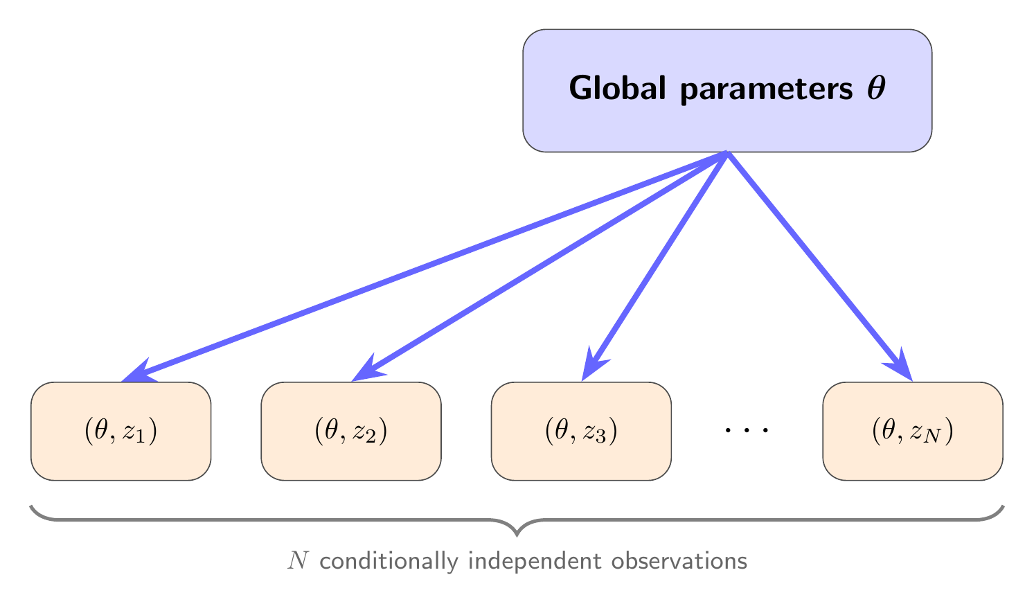] ] ] --- # Example: measuring the expansion of the universe .cols[ .col-1-2[ Type Ia supernovae have a fixed intrinsic luminosity (**standard candles**). The apparent flux depends on the luminosity distance: $F = L / 4\pi d\_L^2$ .small[ **Distance modulus** (the thing that telescopes measure): $$\mu(z) = 25 + 5\log\_{10}(d\_L / \text{Mpc})$$ **Luminosity distance**: $$d\_L(z) = (1+z)\int\_0^z \frac{c}{H(z')}dz'$$ **Hubble parameter** ($\Omega\_\Lambda = 1 - \Omega\_m$): $$H(z) = H\_0\sqrt{\Omega\_m(1+z)^3 + (1-\Omega\_m)}$$ ] .small.muted[Data: [SCP Union2.1](https://supernova.lbl.gov/Union/) — 580 Type Ia supernovae] ] .col-1-2[ .center.width-100[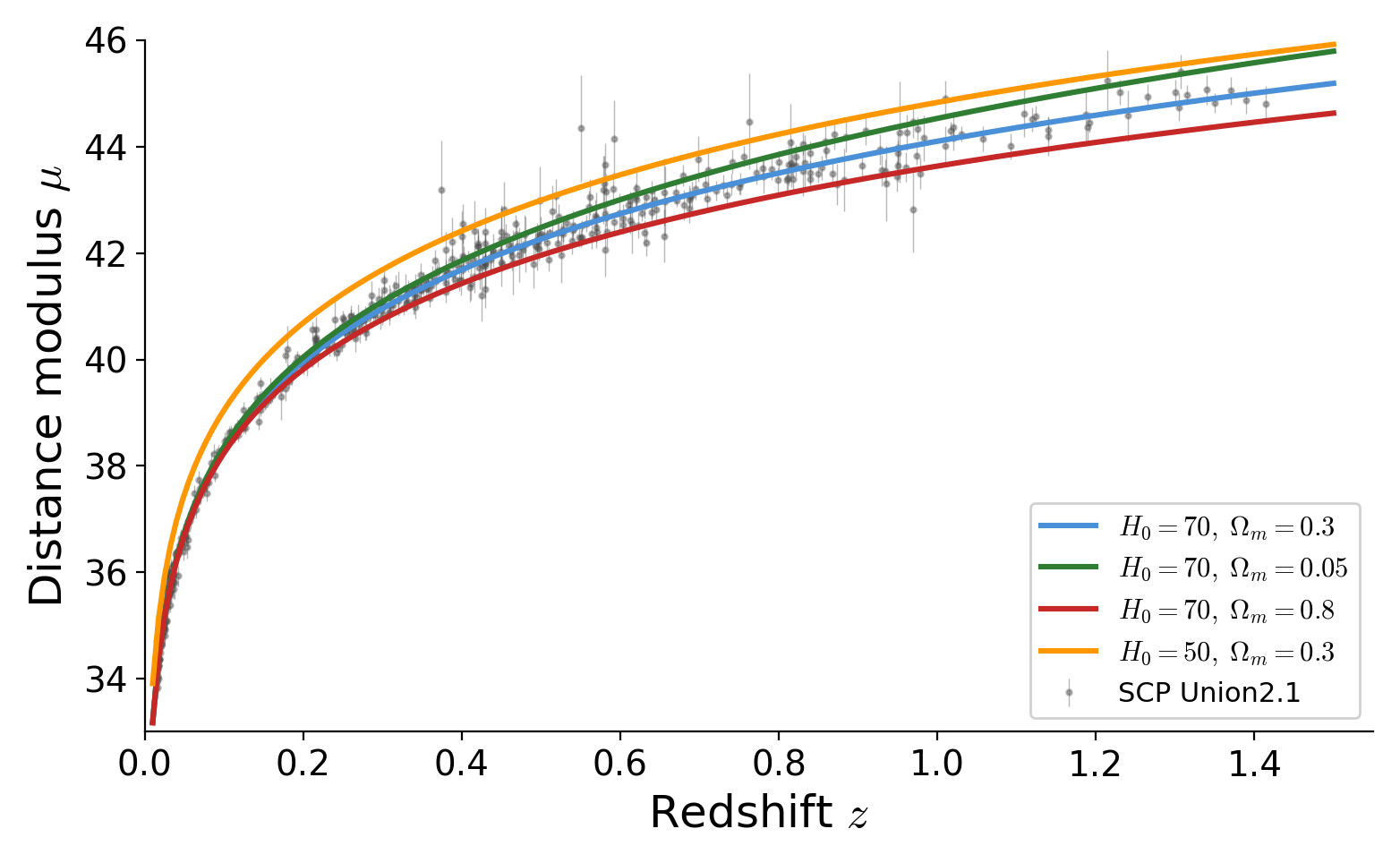] ] ] --- # The supernova model .cols[ .col-1-2[ The **generative story**: 1. The universe has cosmological parameters $\theta = (H\_0, \Omega\_m)$ 2. For each supernova $n$ at known redshift $z\_n$, the **forward model** computes $\mu\_n = \mu(z\_n, H\_0, \Omega\_m)$ by numerically integrating the Friedmann equation 3. Our telescope measures with Gaussian noise: $\mu\_n^\text{obs} \sim \mathcal{N}(\mu\_n, \sigma\_n^2)$ ] .col-1-2[ .center.width-100[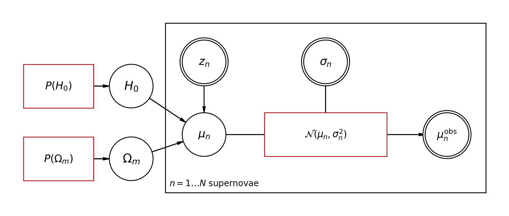] ] ] --- # Supernovae in code ```python def sn_model(z_obs, mu_obs, mu_err): # Shared cosmological parameters H0 = numpyro.sample("H0", dist.Uniform(50., 100.)) Om = numpyro.sample("Om", dist.Uniform(0., 1.)) # Predicted distance modulus for each supernova mu_pred = distance_modulus(z_obs, H0, Om) # Each supernova is an independent observation with numpyro.plate("supernovae", len(z_obs)): numpyro.sample("mu_obs", dist.Normal(mu_pred, mu_err), obs=mu_obs) ``` .small[ `distance_modulus` integrates the Friedmann equations — a differentiable simulator! HMC uses gradients through the entire forward model, including the numerical integration. ] --- # The supernova posterior .cols[ .col-1-2[ .width-100[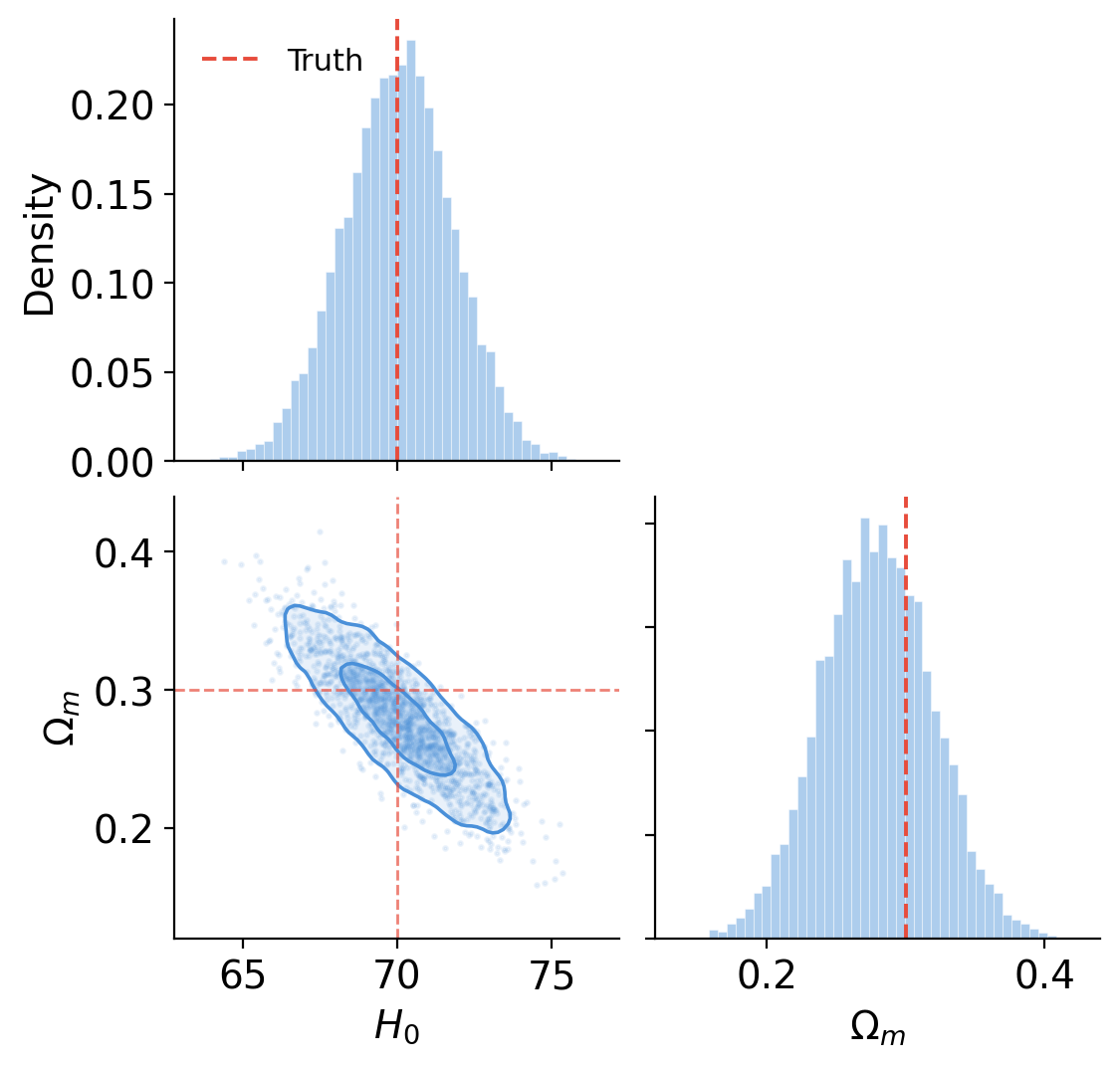] ] .col-1-2[ .width-100[] ] ] .small.muted[Data: SCP Union2.1 compilation of Type Ia supernovae. We'll work through this in the lab notebook.] --- # A more realistic model (Feeney, Mortlock & Dalmasso 2017) Here's the PGM from a full Bayesian distance ladder analysis (~3000 parameters!) .center.width-75[] --- # What if the likelihood is intractable? Many simulators have stochastic internal steps, complex latent structure, or are black-box code. We can run them forward but **cannot evaluate** $p(x \mid \theta)$. .center.width-60[] **Next time — simulation-based inference (SBI):** learn the likelihood or posterior from simulated data.